

SEEFOR 17(2): 26023
Article ID: 26023
DOI: https://doi.org/10.15177/seefor.26-023
ORIGINAL SCIENTIFIC PAPER
Estimating Changes in Structural Attributes within a Repeated-Measurement Framework on Concentric Circular Plots in an Uneven-Aged Dinaric Fir–Beech Stand
Mislav Vedriš1, Nikolina Ušljebrka2, Ivan Bazijanec1,*, Anamarija Jazbec1, Mario Božić1
Addresses:
(1) University of Zagreb, Faculty of Forestry and Wood Technology, Institute of Forest Inventory, Management Planning and Remote Sensing, Svetošimunska 23, HR-10000 Zagreb, Croatia;
(2) American International School of Zagreb, Damira Tomljanovića Gavrana 3, HR-10020 Zagreb, Croatia
*Correspondence: e-mail: ibazijane@sumfak.unizg.hr
Citation: Vedriš M, Ušljebrka N, Bazijanec I, Jazbec A, Božić M, 2026. Estimating Changes in Structural Attributes within a Repeated-Measurement Framework on Concentric Circular Plots in an Uneven-Aged Dinaric Fir–Beech Stand. South-east Eur for 17(2): 26023. https://doi.org/10.15177/seefor.26-023 .
Received: 12 Jun 2026; Revised: 11 Sep 2026; Accepted: 15 Sep 2026; Published online: 6 Oct 2026
Cited by: Google Scholar
Abstract
Field sample plots are the main data source for estimating forest structure. To optimize measurement, nested concentric circular plots are used with plot size depending on diameter at breast height (dbh). Nested design increases efficiency but complicates estimation of temporal change from repeated surveys on the same plots. Twenty-nine sample plots with mapped tree positions at time (t1) were established in an uneven-aged Dinaric fir–beech stand. Two designs were applied on the same plot centres: fixed 20 m radius plots (R20) and concentric plots with radii 7, 13 and 20 m for trees above 10, 30 and 50 cm dbh, respectively (R7-13-20). Data for the second time point (t2) were derived from t1 data by modelling individual-tree increment and ingrowth (dbh threshold: 10 cm) over a 10-year period. Number of stems (N), basal area (G), standing volume (V) and diameter distribution were calculated at both time points. The two methods were compared using paired t-test for N, G, V and chi-square test for dbh distributions. The differences at t1 were minimal: R7-13-20 produced slightly lower estimates of N, G and V that were not proven different (p=0.216; p=0.364 and p=0.535, respectively); the concentric plots at t2 brought higher estimate of N (+88 stems·ha-1, p=0.010), while G and V remained close to R20 (basal area +0.59 m2·ha-1, p=0.625; volume +1.2 m3·ha-1, p=0.934). Differences in dbh distributions were negligible at t1 (p=0.603), but considerable at t2 (p<0.001). The main cause of discrepancy between methods in N and dbh distributions at t2 is the difference in estimated ingrowth (+126 stems·ha-1). The effect of nongrowth trees in R7-13-20 (+24 stems·ha-1 entering the sample via dbh thresholds 30 and 50 cm) was partially offset by survivor trees transitioning over time into larger plot circles (-17 stems·ha-1) due to decreased tree expansion factor (TEF). Observed ingrowth overestimation is a consequence of plot design (high TEF of ingrowth trees) with higher variance, combined with discrete positively skewed distribution of ingrowth (no negative values). In a stand with uneven-sized selection structure with constant regeneration this effect is expected. This type of concentric plot design provides reliable stand-level estimates of N, G and V at a single time point, and stable G and V change estimates, but unstable change estimate of N (particularly ingrowth) over a 10-year period. This inconsistency is expected to diminish over longer temporal scale and larger area (i.e., greater sample size).
Keywords: forest inventory; sampling; nested plot design; terrestrial measurement; stand structure; ingrowth; nongrowth
INTRODUCTION
Reliable information on forest conditions and their changes is essential for long-term forest management planning and sustainable forest management. Forest inventories provide the quantitative basis for assessing stand characteristics and monitoring their development over time (Husch et al. 2003). The quality of an inventory is primarily determined by the accuracy of the estimates and the cost of data acquisition, making inventory design a balance between these two competing objectives. The optimal balance depends on the inventory objectives and the resources available (Schreuder et al. 1993, Mäkinen et al. 2012).
The two principal approaches for acquiring data on forest condition and changes in forest structure are field-based measurements and remote sensing, either applied separately or in combination. Despite substantial technological advances, remotely sensed data alone do not yet fully meet the accuracy and reliability requirements for widespread operational use in forest inventories (Papucci et al. 2026). Therefore, field plot inventories remain the fundamental source of reference data for estimating stand structure for the purpose of forest management planning and silviculture (Schreuder et al. 1993).
Field sample design from aspect of tree inclusion probability can be with equal probability (fixed-area plots) or variable probability sampling, where tree inclusion probabilities increase with tree size (i.e., plot size depends on tree dimensions). The latter comprises two main variants: 1) Bitterlich angle count (or point) sampling (ACS) and 2) nested plots (usually concentric circular plots, CP) design (Kangas and Maltamo 2006). The CP is based on discrete size classes and multiple plot radii (with stepwise change of tree inclusion probability), and ACS has continuous inclusion probability (usually) proportional to tree basal area.
Regarding plot shape, circular plots are the most commonly used in forest inventory for several reasons: 1) fewer borderline trees (due to smallest perimeter for a given area) directly leading to fewer checks and also fewer measurement errors; 2) simple plot establishment (because of single control point – plot centre), 3) easier determination of individual tree positions (very important on permanent plots) (Shiver and Borders 1996, McRoberts et al. 2015).
Concentric circular plots (CP) that can be tracked to the first half of 20th century in USA (LaBau et al. 2007), and became common in the second half (Austria, Switzerland, France, Germany…) mostly in NFI (Gschwantner et al. 2016). Their key advantage is efficiency attained by well balancing inventory costs and results – allocating the measurement effort on larger trees leads to better estimates of stand basal area (and volume). CP design is especially suitable for stand structures with wide range of tree sizes, such as selection forests (Schreuder et al. 1993). On the other hand, like ACS, they provide less reliable estimates of stand density (Scott 1990), and, consequently, of diameter distribution (Nanos and Sjöstedt de Luna 2017). Concentric plots can also be regarded as more complex than fixed ones for field work, and in some situations leading to many checked (measured) trees that are not included in the sample (thus reducing the efficiency). Since fixed plots are reliable and efficient for estimating stand density, and Bitterlich ACS for basal area and volume, concentric plots are often recommended as a good compromise between these two (Henttonen and Kangas 2015). The applicability of the CP design depends on the target variables and the purpose of the inventory. Although its suitability for estimating structural attributes is well established, concentric plots appear to be less stable for estimating attributes related to biodiversity (Kománek et al. 2024, Moreno-Fernández et al. 2024).
Concentric plot design is known to produce higher variance of estimates which is a result of variable inclusion probabilities and which can lead to substantial differences when compared to fixed plots in finite (especially small) sample. However, it is theoretically not biased in expected values if correct design-based probabilities (Horvitz–Thompson estimators) are used for estimation in single or periodic consecutive sampling (Gregoire and Valentine 2008).
In order to get reliable estimates of stand structure, the sample design must be unbiased. When estimating change of stand attributes, compatibility between two consecutive inventories is a key issue, with additive components of change that sum to the difference between values in t1 and t2 (Meyer 1953, Thompson 2006). Those two aspects are well elaborated (Martin 1982, Eriksson 1995, Gregoire 1995) and applied in forest inventory research and operational inventory programmes (Roesch 2007). Remeasurement on the same plots improves additivity of change estimators and facilitates unbiased estimation of change components (Schreuder et al. 1993).
Generally, the temporal change can be classified into three main components: 1) natural increase (due to tree growth); 2) decrease (mortality and harvest) and 3) estimation issues due to sample design and measurement. Basic concept of change components is expressed by Meyer (1953) and Beers (1962), and has been further developed and adapted for different sampling designs, mostly in the context of ACS (Grosenbaugh 1958, Van Deusen et al. 1986, Roesch et al. 1989, Eriksson 1995)
Given that concentric plots can be regarded as a simplified form of horizontal point sampling with a finite number of plot circles (Gschwantner et al. 2024) they present an intermediate design between fixed plots and Bitterlich ACS. The change components of variable probability designs are more complex than fixed plots due to substantial change of tree inclusion probability over time. In this sense, concentric plots are more similar to ACS, where effects of variable tree inclusion probabilities lead to change in tree expansion factor (TEF) over time (Hébert et al. 2005). When compared to fixed area plots, there are two additional change components: a) larger trees entering the sample and b) decrease of TEF for survivor trees (Kangas and Maltamo 2006). These two effects are present for both variable probability designs with a difference: in CP these changes are stepwise over diameter at breast height (dbh)/distance thresholds while ACS has continuous (large) tree inclusion and decrease of TEF.
Larger trees that enter the sample over higher dbh thresholds present a positive change component, while existing (survivor) trees that shift to larger plot induce negative component in per hectare estimates over time. Although these components partially mitigate (or obscure) each other, they cannot be ignored and should be considered in each inventory.
The complexity of change components in variable plot probability sampling was addressed by many researchers from theoretical and practical view (Shiver and Borders 1996, Kangas and Maltamo 2006, Gregoire and Valentine 2008, Eastaugh and Hasenauer 2013) and has largely been overcome through use of appropriate change estimators (Scott 1990, Roesch et al. 1991, Thompson 2006). Comprehensive research and development of reliable estimators have been made, mostly deriving from ACS methods (Iles and Beers 1983, Van Deusen et al. 1986, Roesch et al. 1989, Hradetzky 1995), while studies concerning CP are rare (Roesch 2007). The effects of changes in tree inclusion probability associated with concentric plot designs are a consequence of diameter thresholds and corresponding subplot radii that influence the representation of individual diameter classes (Gregoire and Valentine 2008). However, these effects have mostly been considered at a conceptual level, while quantitative assessments of their influence on repeated measurements of the same plots remain scarce. In this study, these effects were quantified using the same sample plots across two inventory occasions, allowing changes related to tree inclusion probabilities to be distinguished from actual changes in stand attributes. Although the differences between the fixed and variable area plots have been studied, and theoretical solutions and appropriate estimators have been developed, the application and validation are always needed to quantify the effect of sampling design for any specific forest structure (e.g., Vedriš et al. 2009).
The aim of this study is to compare the estimates of stand structural attributes and their changes obtained from repeated measurements using two types of circular sample plots. Using data from sample plots established in an uneven-aged silver fir–beech stand, this study analyses the estimates of stand structural attributes (N, G and V) and diameter distribution, as well as their changes over time, by comparing triple concentric circular plots with single fixed-radius circular plots. Change between two measurement occasions (for both methods) is additionally analysed by components (increase and decrease):
- increase due to growth of trees on plots and ingrowth of new trees over the dbh thresholds,
- decrease of per hectare N, G and V values due to transition of individual trees to larger plot size (for CP).
- This approach quantifies components of change based on real plot data that enable investigation of the effect of plot design on ingrowth and changing inclusion probabilities inherent to CP design.
MATERIALS AND METHODS
Study Area
The study was conducted in the Gorski Kotar region, Croatia. The area is characterized by a pronounced mountainous karst relief, with average elevation about 800 m a.s.l., which determines a moderately warm and humid climate without a pronounced dry season. The mean annual precipitation is approximately 2000 mm, with a relatively uniform distribution throughout the year. The mean annual temperature is slightly above 7°C, with pronounced temperature extremes, frequent frost occurrence, and very high air humidity. The region is dominated by Dinaric silver fir–European beech forests, characterized by uneven-aged and mixed-species stand structures with a wide range of tree diameters, resulting from the interaction of topographic and climatic conditions and selection forest management system (Bončina 2011). The target structure of uneven-aged selection stands consists of trees of different dimensions, with a characteristic reverse J-shaped diameter distribution. Such a structure is maintained through periodic selection interventions that simultaneously regulate stand regeneration, tending, and harvesting, thereby ensuring continuous forest cover and sustainable yield (Čavlović et al. 2006, Božić et al. 2011).
The selected stand for this research is compartment 10a of the Delnice management unit, managed by the Delnice Forest Administration, and covers an area of 32.59 ha. The stand is situated at an elevation of 900–970 m a.s.l. and represents a typical silver fir–European beech forest association on a limestone substrate (Omphalodo-Fagetum Tregubov 1957 corr. Marinček et al. 1993). It is characterized by an uneven-aged stand structure, a significant proportion of silver fir, and long-term management under the selection system.
Data Collection and Analysis
Two plot designs (methods) are evaluated in this study. The first is a fixed-radius circular plot with a radius of 20 m (hereafter R20), which was used as the reference design. The second is a three-radius concentric plot design with radii of 7, 13, and 20 m (hereafter R7–13–20), designed for Croatian national forest inventory (CRONFI; Čavlović and Božić 2008). Size and dbh thresholds in R7-13-20 are defined as follows (Figure 1):
- plot radius 7 m (area 153.94 m2) for measuring trees with dbh ≥10 cm,
- plot radius 13 m (area 530.93 m2) for measuring trees with dbh ≥30 cm,
- plot radius 20 m (area 1256.64 m2) for measuring trees with dbh ≥50 cm.
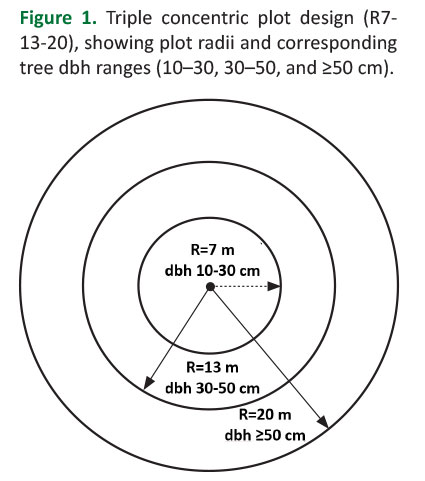
Data for first inventory (t1) were collected on 29 field plots established on a systematic square grid with a spacing of 100 m between adjacent plots. On circular plot with radius 20 m trees were measured for dbh, distance, azimuth and slope to the plot centre. At each sample plot, tree heights were measured on a subsample of trees.
Tree diameters were measured for all trees with a minimum dbh of 10 cm. Diameter measurements were taken at 1.30 m above ground level using a Haglöf Mantax calliper with 1-mm graduations. The horizontal distance and azimuth were measured from the plot centre to the central vertical axis of each stump. Distances, slope, and tree heights were measured using a Vertex IV ultrasonic hypsometer/rangefinder with a transponder, while azimuths were determined using a Suunto KB-14 compass.
The volume of each individual tree was calculated using the back-transformed Schumacher–Hall equation (Equation 1):
v = a × dbhb × hc × f (1)
where v is tree volume; dbh is diameter at breast height; h is total tree height; a, b, and c are species-specific regression parameters (Špiranec 1975, 1976); and f represents Meyer’s correction factor (Schumacher and Hall 1933). The measured tree heights were used to model the stand curve using the Michailoff equation (Michailoff 1943) and height of each tree was calculated as (Equation 2):
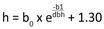 (2)
where h denotes modelled total tree height, b0 and b1 are species-specific model parameters, and dbh represents tree diameter at breast height.
The tree data for the R7–13–20 were derived from the R20 plot data using the recorded tree diameters and distances from the plot centre by applying the concentric sample plot criteria (Figure 1).
In order to get per hectare values, TEF was applied, depending on the plot size (TEF = 1/plot size). Such calculation was performed for each tree and each attribute (number of stems, basal area and volume) resulting in per-hectare values of N, G, V. Plot estimates are sums of all trees on individual plot and stand level value was estimated as an average of all plots.
The spatial pattern of trees on R20 plots was analysed using the Clark–Evans index (Clark and Evans 1954) with the edge-effect correction proposed by Donnelly (1978).
The second inventory plot data (t2) were derived from the initial measurement (t1) after a 10-year projection period for both sampling designs. Diameter increment of the existing (survivor) trees was estimated using a linear growth model developed from repeated measurements of tree diameters within the FirGroDin project (Impact of Forest Management and Climate Change on the Growth Dynamics of Silver Fir Trees and Stands in the Dinaric Region of Croatia; Božić et al. 2025). In addition to the growth of survivor trees, tree recruitment (ingrowth) was simulated, defined as trees exceeding the inventory threshold of 10 cm dbh during the 10-year interval. The number of trees in the 5–10 cm dbh class at t1 was estimated for each sample plot using a simple regeneration model based on the expected stand density for the corresponding forest type (100 trees·ha⁻¹ at full stocking, adjusted by the stand relative volume-based stocking factor; Čavlović 2013), the diameter distribution, and the predicted diameter increment of individual trees.
Estimate of change for each structural attribute (N, G and V) was made for each sampled tree (Equation 3):
∆Xi = x2i × TEF2i - x1i × TEF1i (3)
where ΔXi is change in per hectare value of each stand attribute (x meaning N, G, or V) as contribution of i-th tree, TEF is tree expansion factor, and indices 1, 2 standing for time points t1 and t2.
The contribution of each tree was classified depending on the change of its status in t2 as follows (adapted from Martin 1982, Hasenauer and Eastaugh 2012):
- survivor – trees that were sampled at t1 and remain in sample at t2 without changing its status;
- ingrowth – (small) trees that enter the sample in t2 by reaching dbh threshold 10 cm;
- nongrowth – trees that were present in stand at t1, but enter the sample only in t2 by reaching the higher dbh threshold and distance from plot centre (nongrowth 2 – dbh over 30 cm within 13 m radius, nongrowth 3 – dbh over 50 cm within 20 m radius); it is equivalent to the ingrowth for higher thresholds (30 and 50 cm) and valid only for R7-13-20;
- transition – trees that were sampled at t1, remain in sample at t2, and due to radial growth and crossing the dbh threshold 30 or 50 cm are reassigned to the larger circle (transition 2 – over 30 cm, transition 3 – over 50 cm); only for R7-13-20.
The calculation of changes between the two measurement occasions (t1 and t2) excluded natural mortality and harvest, in order to better demonstrate these effects of CP sampling design: nongrowth trees and the artificial transition of trees due to changes in plot inclusion status.
Paired t-test with significance level 0.05 was used for comparing average values (N, G and V) between two methods at each time point (t1 and t2).
Since greater differences between methods can be expected for stem density (N·ha⁻¹), owing to differences in the probability of tree inclusion and the inherent characteristics of this variable (Shiver and Borders 1996), diameter distributions derived from two methods were compared at t1 and t2. Diameter distributions were made by grouping trees in 5 cm diameter classes (multiplied by TEF to obtain per hectare values). For testing the differences between distributions chi-square test was applied (Sokal and Rohlf 1995), with relative frequencies of R20 used as reference for expected values of R7-13-20, and observed frequencies rounded to whole number values.
RESULTS
Differences between Methods at Two Time Points
Estimates of stem density (N), basal area (G) and standing volume (V) by the two methods at both measurement occasions (t1 and t2) are presented in Table 1.

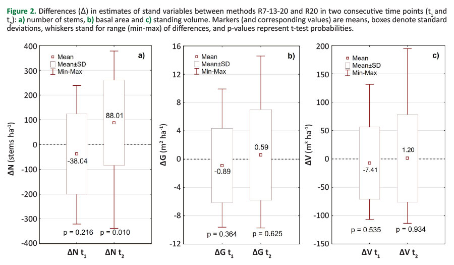
The biggest difference between method averages is in stand density (N) at both time points. Method R7-13-20 shows higher variability for all three variables at both time points, with standard deviation of N being considerably higher than R20. The more detailed comparison of methods is shown in Figure 2.
Method R7-13-20 showed lower estimates of N, G, V in t1, and higher in t2, when compared to R20 (Table 1, Figure 2). While G and V differences are minimal, number of stems shows considerable discrepancy between methods, especially in t2, where the difference was statistically significant (p = 0.010, Figure 2).
Variability of differences is larger in t2, as well as extreme (positive) ones, as can be seen from Figure 2.
The observed plot CE values range from 0.7–1.07 (average 0.95) and indicate spatial patterns very close to random, with only weak departures towards either aggregation or regularity. Most plots show almost random pattern (CE between 0.95 and 1.05), some are aggregated and only two plots show slight regularity tendency (CE over 1.05).
Differences between Methods on Individual Plots
Although both methods use the same plot centres, differences between their estimates arise from differences in tree inclusion probabilities associated with the respective plot designs. This effect was observed at the stand level and was even more pronounced at the individual plot level. The most extreme differences between methods for all stand attributes at t1 and t2 were identified and are presented in Figure 3 and 4.
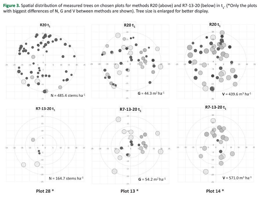
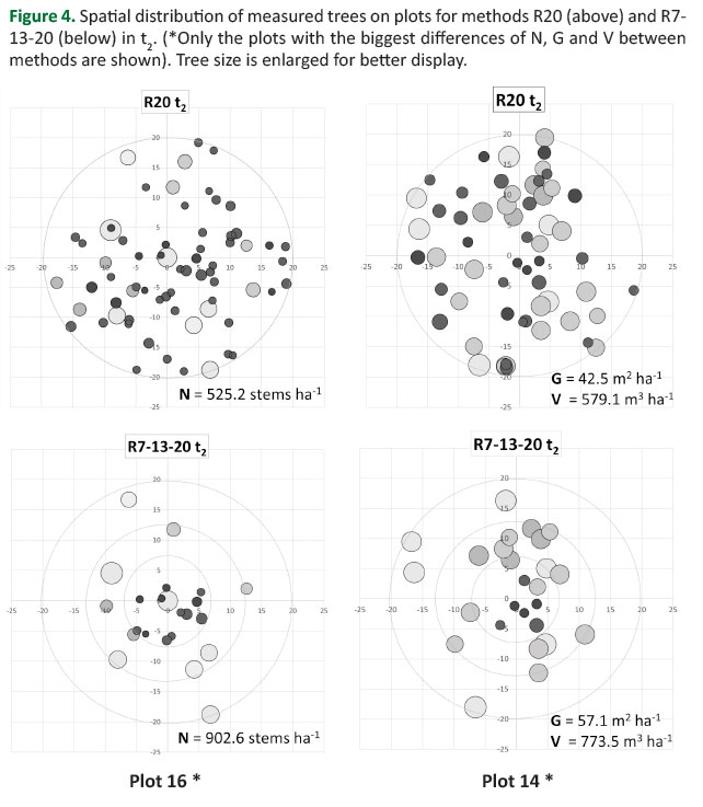
When looking on the individual plot level, differences in estimate of N between methods are related to the spatial distribution of trees, especially the smaller ones: plot with small trees (10-30 cm dbh) grouped around plot centre leads to large estimate on R7-13-20 (plot 16, Figure 4), and plot with no smaller trees within 7 m radius has lower estimate than R20 (plot 28, Figure 3). Both plots have slightly aggregated spatial pattern of trees (CE index 0.98 and 0.96, respectively). The biggest differences in estimates of G and V between methods on plot-level are consequence of (the same) middle sized trees (30-50 cm dbh) within 13 m radius, that make higher per hectare estimates by R7-13-20 due to greater TEF (18.83 vs. 7.96 for R20) on plot 13 and 14 (Figure 3 and 4). Plot 13 has slightly aggregated pattern (CE = 0.93), while Plot 14 has (highest) CE index (1.07) indicating regular pattern with considerable share of medium sized trees.
Diameter Distributions
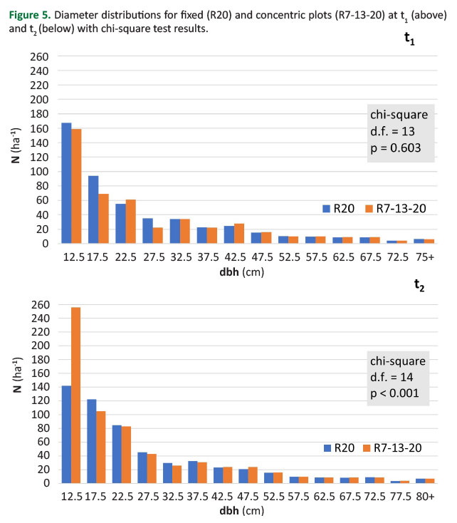
The diameter distributions obtained by the two methods are very similar at t₁ across all dbh classes, with no statistically significant overall difference (Figure 5, above). At t₂, both methods showed the expected increase across most dbh classes; however, a pronounced divergence was observed for trees in the 10–15 cm dbh class. In this class, the R7–13–20 method resulted in an almost twofold higher estimate of N·ha-1 compared with R20, indicating a discrepancy in estimated ingrowth and leading to the statistically significant chi-square test result (Figure 5, below).
Temporal Change between Two Time Points
To better analyse the methods, changes in each structural attribute between t₁ and t₂ are presented by their components of change (Figure 6).
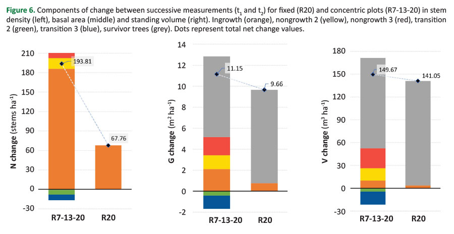
The greatest difference between methods is in change estimate of N (126 trees·ha-1, Figure 6 left) as was also indicated by average estimates in t1 and t2 (Table 1, Figure 2). The ingrowth is the largest component of net change for R7-13-20 (96%), followed by trees crossing thresholds 30 and 50 cm (nongrowth, 13%). The nongrowth effect is partially offset by trees transitioning to larger plots (transition 2 and 3, around -9%). For R20 the ingrowth is the only effect of N change (since there was no mortality nor harvest).
The main effect of basal area change for both methods comes from survivor trees (around 69% and 92%, respectively). For method R7-13-20 ingrowth effect is substantially less for basal area than for number of stems, but it contributes basal area change with 19%. Trees crossing the 50 cm threshold (nongrowth 3) make around 16% of basal area change. The main contribution to volume change for R7-13-20 are survivor trees (79%), followed by nongrowth 3 (17 %) and nongrowth 2 (11%), while ingrowth makes only 7%. Transition trees in R7-13-20 make around -15% of change in G and V, compared to -9% for N (due to their greater "weight" for G and V than for N). The ingrowth component for R20 makes 8% of basal area change, and only 2.5% of volume.
Temporal Change by Plots for Concentric Plot Design
Since method R7-13-20 is less consistent, has a higher variability (especially for N·ha-1, Table 1), and also has more complex change components, changes of N·ha-1 are analysed on individual plot level for CP design (Figure 7).
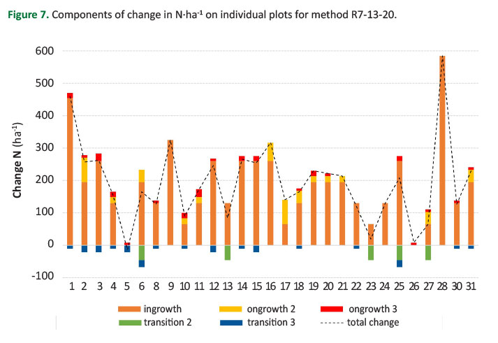 Figure 7. Components of change in N∙ha-1 on individual plots for method R7-13-20.
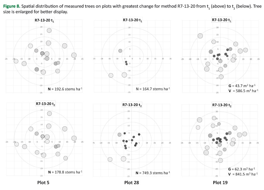
Plots with most extreme values of N change (5 and 28) are further examined, in addition with plot 19 that showed greatest change of G and V (Figure 8).
Only plot 5 showed a negative net change between t1 and t2, due to a combination of the following effects: two trees transitioning from circle 2 to 3 (decrease of TEF from 18.83 to 7.96) and no ingrowth or nongrowth trees (Figure 8, left). Plot 28 has highest increase in stem density (584.6 trees·ha-1) due to as many as nine ingrowth trees located close to plot centre (within 7 m radius, Figure 8, middle). The highest increase in G and V, recorded on plot 19, is resulting mainly from growth of (large) survivor trees and enhanced by three nongrowth trees entering the sample over thresholds 30 (1 tree) and 50 cm (2 trees) (Figure 8, right).
Ingrowth Estimates
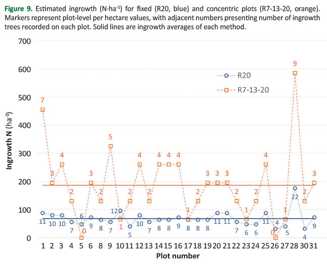
Since the estimated ingrowth is detected as the main source of differences between methods for stem density (N·ha-1) at t2 (Figure 5, below), the per plot ingrowth values for both methods are presented in Figure 9. The average ingrowth is almost triple on R7-13-20 compared to R20 (185.9 vs. 67.7 trees·ha-1, Figure 9), with individual plot values varying from 0 to 584.7 trees·ha-1 (R7-13-20) and 31.8 to 175.0 (R20).
Although R7-13-20 has two plots without ingrowth (and no such plots for R20), its average is considerably higher due to extreme positive values (584.7 trees·ha-1 on plot 28, Figure 9). The data from this figure also show considerably higher variability of per plot ingrowth estimates in method R7-13-20 compared to R20.
Since the ingrowth occurs on the whole plot area of R20, and only on smallest circle (r = 7 m) in R7-13-20, there is evident effect of (large) TEF. Method R7-13-20 has approximately eight times larger TEF than R20, leading to equivalent ingrowth per ha by two methods estimated on plot 17 with single ingrowth tree in R7-13-20 vs. 8 ingrowth trees on R20. The opposite example is plot 28 with 22 trees on R20 and 9 on R7-13-20 that resulted in three times higher estimate per ha (Figure 9).
DISCUSSION
In this study the two plot designs were compared for estimation of stand structure, where R20 was used as reliable design due to the large inclusion probability, covering large area and including many measured trees, with plot size being around the upper limit for practical field plot establishment (Jazbec et al. 2011, Kománek et al. 2024). The reliability of R20 was confirmed by Jazbec et al. (2011) who showed that the precision of estimates stabilizes up to plot radius 20 m in the same forest type. Larger plots would not be practical due to large number of trees, restricted visibility, more checking of borderline trees. The other method (R7-13-20) was used as an example of comparably large triple concentric plot design common in large scale inventories (Gschwantner et al. 2016). It should be noted that none of these methods is used as standard in a stand-wise inventory. Plots with 20 m radius are not used in inventory practice in Croatia due to practical reasons (average 62 and 71 measured trees per plot at t1 and t2) and were considered the reference value in the absence of a total census (Brooks and McGill 2004), while R7-13-20 was originally developed for CRONFI as a standardized sampling configuration applicable to all forest types on the state level (Čavlović and Božić 2008).
The proposed approach for comparison was aimed to present clear effect of plot design on stand level by in-depth analysis of differences on plot- and tree-level contributing to overall estimates of stand attributes and their change. Although in real inventory conditions temporal change includes also harvest and/or mortality, it was not presented in this research in order to present more clearly the "negative growth" effect of CP method, the similar approach used by Beers (1962). Observed "negative growth" effect on single plots with CP method due to transition would be mostly obscured if mortality and harvest were included. Real inventory data are inevitably burdened with measurement errors (Božić et al. 2025) that would bring additional "noise" in results and were therefore eliminated in this research.
The investigated uneven-aged stand structure very well accents the difference between methods in estimating stem density, that would be less prominent in even-aged (especially older) stands with negligible ingrowth. Furthermore, stand level used (29 sample units) presents a sample small enough to be sensitive to plot-level extremes (e.g., plot 28), which would even out on a large scale.
All observed effects (especially the discrepancies) would be hard to detect and measure, and impossible to analyse (or explain) without available reference value (20 m radius plots in this case).
Estimating change between two consecutive inventories can be made on two levels: total change on a stand or higher level and growth of individual (or average trees) between two time points. Estimators for fixed plots are simple since there is no change of TEF over time. For variable probability design (ACS and consequently CP) due to the TEF change more complex estimators have been developed (Van Deusen et al. 1986). Our results well represent the practical outcomes of these change components.
When calculating temporal changes using permanent CP (nested design), as well as ACS, there are two basic approaches. In the first approach, TEF for each tree depends on the plot radius to which the tree belongs in the current measurement. This approach is simpler and provides an unbiased and more accurate estimate of stand status at each measurement occasion. In the second approach, TEF for each tree is calculated according to the plot radius to which the tree belonged in the first measurement. This approach is more appropriate for an exact estimation of tree- and plot-level increment, but it is more complex and may introduce bias when used for estimating the overall stand status (Scott 1990). This study used the first approach and the change estimator used in this study follows the concept of Van Deusen et al. (1986) and Roesch et al. (1989), where per-hectare estimates of tree number, basal area and volume are calculated for individual trees at each remeasurement occasion (using appropriate TEF), aggregated at the plot level, and change is subsequently expressed as the difference between plot-level estimates. Therefore, our results show the expected inconsistency at the individual plot level due to changes in TEF inherent to CP for N·ha-1 (e.g., plot 5) as also demonstrated by Božić et al. (2025) for basal area and volume.
Because the sample size was identical for both methods, variability expressed as standard deviation was directly proportional to the standard error. Therefore, standard deviation was considered an appropriate measure for comparing the relative precision of the two methods.
The average stand-level estimates of all G and V were consistent for both methods at both time points, with CP design resulting in slightly higher variability (consequently, less precision, Table 1). The t1 estimate of average N by CP method corresponded to R20 at t1, with as much as twice higher variability (and error of estimate). However, the estimate of N at t2 was proven different between methods, and particularly the estimated change between t1 and t2, revealed the instability of the CP method associated with considerably higher variability (the standard deviation for R7–13–20 was more than twice that of R20; Table 1). This is in accordance with statement from Martin (1983) that fixed plots are always more precise than ACS for attributes not correlated with basal area. Our results are generally in line with previous findings from different forest conditions for ACS (Scott and Alegria 1990) that variable-radius plots are better for stand attributes associated with large diameter trees and less efficient (due to variability) for estimating attributes concentrated in the small diameter classes (Schreuder et al. 1993).
For the R7–13–20 method, an apparent overestimation of the change in N was observed, which was subsequently identified as resulting from differences in the estimation of ingrowth trees (Figure 5, 6, 9). Since the ingrowth model (simulated recruitment of trees below the 10 cm diameter threshold) was defined as a spatially random distribution and the plot-level estimates were correctly weighted by using TEF, this pattern cannot be attributed to systematic error or bias in the estimation of ingrowth caused by tree spatial distribution. Furthermore, this effect is not related to measurement error (plot edge effect), as this potential source of bias was excluded due to the nature of t2 data in our study. Although the R7–13–20 method has diameter thresholds (dbh = 30 and 50 cm) for tree inclusion in the two larger concentric circles (r = 13 and r = 20 m), these trees do not cause a substantial increase in estimate of stem density due to the natural dynamics of uneven-aged stand structure and the reverse-J diameter distribution, where substantially more trees are crossing the 10 cm threshold than the 30 and 50 cm thresholds. The values of these three categories (ingrowth, nongrowth 2 and 3) are appropriately expressed per hectare with adequate tree expansion factors, and the ingrowth considerably exceeds nongrowth for N (Figure 6, left).
However, the effect of nongrowth becomes more pronounced for G and V because it involves larger-diameter trees with substantially higher individual contributions to basal area and volume estimates (Figure 6, middle and right). Unlike N, where all trees contribute equally to the total or mean estimate regardless of their size, changes in G and V are weighted by tree dimensions. Consequently, ingrowth has only a minor effect on G and V, whereas transition and nongrowth contribute more substantially due to the greater size of the involved trees (Figure 6).
When analysing the overestimated number of ingrowth trees on CP, it can be attributed to the plot size and nature of ingrowth variable. Plot size can play a significant role in two ways. First, although any plot size can have plots without ingrowth trees, it happens more often on smaller plots (due to lower tree inclusion probability). In our example "ingrowth plot" has radius 7 m in CP (compared to 20 m in fixed), leading to 2 "zero ingrowth" plots in R7-13-20 and none in R20 (Figure 9). However, this effect did not have a substantial influence on the overall per hectare values. Second, small plot has significantly higher TEF (64.96 for R7-13-20 compared with 7.96 for R20), resulting in greater weight of each tree recorded on the 7 m plot. Finally, the discrete and non-negative nature of ingrowth variable (values 0,1,2…) in combination with effect of large TEF has led to extreme estimates on individual concentric plots (with no possible negative balance) leading to higher variance, and (in our case) overestimation of average value for ingrowth (Figure 9) and total N change (Figure 6) when compared to R20. Partial compensation of increase from ingrowth on R7-13-20 is due to transition: some trees "exit" from 7 m circle and shift to a larger plot (r = 13 m) with smaller TEF, thus reducing per hectare value. However, they are fewer than ingrowth (due to stand structure explained above) and consequently transition effect is considerably less than ingrowth (Figure 6). From the perspective of plot design, our results indicate that the small plot radius was the main cause of the instability in estimating the number of trees in the studied forest type. It is important to note that this effect is not inherent to the concentric-plot design and would equally occur with a fixed-radius plot of the same size (Brooks and McGill 2004, Jazbec et al. 2011). This interpretation is supported by the findings of Moreno-Fernández et al. (2024), where some rare tree species were absent from the concentric-plot sample because they were represented by small-diameter trees that were not included in the smaller-radius plots when located farther from the plot centre.
The higher variability on R7-13-20 in combination with the relatively small number of simulated plots and the short simulation period (10 years), resulted in a higher observed mean ingrowth N estimate in this study. This apparent overestimation reflects sampling variability rather than a systematic bias, as unbiased estimators may produce estimates above or below the expected value in individual samples (Cochran 1977). Therefore, with an increasing number of plots and/or a longer observation period, the mean estimates of ingrowth, and consequently N, obtained by the R7–13–20 and R20 methods are likely to approach the same expected value. The practical problem on the stand level however, exists, and R7-13-20 should be taken with caution in estimates of ingrowth or small diameter trees generally. It should be noted that the observed instability (apparent overestimation) of the estimated stem density is not inherent to CP alone (it is even partially compensated by transition to larger circle, Figure 6) but rather represents a general consequence of small plot sizes. Consequently, small plots combined with a small sample size may produce unreliable estimates of ingrowth. Therefore, plots with radii larger than 7 m are preferable for obtaining more reliable estimates of ingrowth, particularly in uneven-aged stands, where continuous recruitment of small-diameter trees is essential for maintaining the uneven-aged stand structure (Čavlović et al. 2006), especially when regeneration is irregular or insufficient (Teslak et al. 2016).
Compatibility (or additivity) of change estimates is generally requested as a key issue in (permanent) inventory design. It is required from theoretical point of view and also from the users of inventory results – incompatible estimates lead to lack of reliability (Van Deusen et al. 1986). However, in real conditions additivity may be impossible to achieve due to changes in (forest) land area and/or sampling design. These two issues usually make greater effect than changes in tree inclusion probabilities that were covered by our research, especially in large area forest inventories (Schreuder et al. 1993). In such cases increased complexity of estimators to ensure additivity may not be justifiable (ibid.). Insisting on additivity is reasonable when tree-, plot- or stand-level estimates are important and detailed calculations such as presented in this paper can be performed. To ensure additivity of estimated change on plot level, possible adjustment is to use only survivor trees on the same plot size from consecutive inventories (e.g., Talarczyk 2014) for net increment.
Although the two-sample Kolmogorov–Smirnov test is commonly used to compare diameter distributions (Bončina et al. 2022), it was not applicable in the present study because the compared samples were not independent (Conover 1999). Since the concentric-plot data were derived from the fixed-radius plot data, they represent a subsample of the R20 plots, and such a comparison would not be appropriate. Even if independence could be achieved by comparing the R7–13–20 trees with the excluded-tree sample, the resulting comparison would not be meaningful because the sampled trees in the R7–13–20 have, by plot design, larger dbh on average than those included in the R20 sample. In contrast, the chi-square test was appropriate because the comparison was performed on diameter-class distributions scaled to a per-hectare basis. This standardisation enabled comparison of the estimated dbh distributions derived from the two methods, rather than direct comparison of the original tree diameters. Comparison of dbh distributions did not reveal a significant difference at t1, while a statistically significant difference at t2 resulted solely from trees 10–15 cm dbh (ingrowth, Figure 5) as was also reflected in the differences in mean values (Figure 2).
The observed slightly aggregated pattern (average CE = 0.95) is expected in uneven-aged stand structure where selection forest management is applied, with sporadic (small) groups of young trees. Some differences (between methods or change on R7-13-20) observed on individual plots can be attributed to spatial arrangement of small trees (and ingrowth trees), but the major differences cannot be generally explained by spatial distribution of trees, due to relative consistent CE index between plots and not clear correlation of extreme differences with CE. It can indirectly be related with the grouping of smaller trees that make key difference in estimating N·ha-1 (small trees close to plot centre on plot 16 or absence on plot 28, also with large ingrowth in t2). The largest differences in G and V between methods are observed on plot 14 that shows most regular pattern (CE = 1.07) and has a significant share of middle-sized trees (Figure 3 and 4). Under clustered spatial patterns (CE < 1), different plot designs at the same plot centres (and even more so at different points) are more likely to include different tree groups because of differences in their inclusion zones. Consequently, greater discrepancies among plot designs are expected than under random or regular spatial patterns (Gregoire and Valentine 2008).
The choice between fixed or variable (ACS or CP) probability designs primarily depends on type of inventory, regarding the spatial scale and inventory objectives. It is further based on the importance of forest attributes, stand structure, available funds and field personnel (survey crews). The combinations of ACS and fixed plots provide such unbiased and practical possibility (e.g., Berger et al. 2020, Leiter and Hasenauer 2023). The CP design has similar effect of balancing the field effort and quality of estimates (Henttonen and Kangas 2015), where the number and size of the circles should be adjusted to above-mentioned real circumstances. Although plot design can be theoretically adequate or optimal, actual field conditions must be taken into account. For instance, the borderline trees, whose influence has been minimised in our study, represent a serious source of errors (missing trees). In that sense, although larger plots are generally more adequate for uneven-sized and uneven-aged stands, the number of borderline trees increases with increasing plot radius. Despite the error of each missing tree decreases with larger radius due to larger TEF (Rodríguez-Ruiz et al. 2025), the problem of less visibility (obscured trees) increases (Husch et al. 2003). Missing distant trees can be mitigated by applying a truncated plot radius, often combined with ACS design (Poso and Waite 1995, Berger et al. 2020).
In this study we adopted CP design from CRONFI to check its performance on a stand level. However, for stand-level forest inventory, the radii of the concentric plots could be optimized according to stand structure. The observed instability of estimated ingrowth suggests that the radius of the innermost concentric plot should be increased. For example, increasing the radius of the smallest concentric plot from 7 to 9 m (254.5 m²) would increase the average number of measured trees by approximately five per plot, including about one additional ingrowth tree. At the same time, the tree expansion factor (TEF) would be reduced by nearly 40%, which would be expected to decrease the variability of ingrowth estimates and improve the precision and stability of the estimated number of trees. When compared with the reliable fixed circular sample plot well-established in operational forest inventories in Croatia (radius 12.62 m; area 500 m²), the proposed plot size (e.g., r = 9 m, Vedriš 2010) would require substantially fewer tree measurements per plot. The resulting reduction in field effort could therefore be reallocated to increasing the plot area for medium-sized (dbh 30–50 cm) and large trees (dbh ≥ 50 cm) by extending the radius of the outer concentric plot to 14 m or more, depending on stand conditions, as suggested by Vedriš (2010). Such a two-radius nested plot design (e.g., 9-14 m) would also be more practical from an operational perspective, since it simplifies field measurements and is easier to implement than three-radius configuration (Dvorak 2000). Such a design may provide a better balance between field efficiency and estimation precision than triple circles while still being more flexible than the single-radius plots currently used in operational forest inventories in Croatia.
CONCLUSIONS
This study compared the estimation of stand attributes from repeated measurements using concentric and fixed-radius field plots. The applied concentric plot design from the Croatian National Forest Inventory provided similar estimates of basal area and volume (G and V) to those obtained from 20 m radius plots at the stand level at two individual time points. The results of two opposing components of change in concentric plot design — the entry of larger trees into the sample (nongrowth) and the decrease of number of stems, basal area and volume per hectare due to the larger plot area assigned to individual trees in the second measurement (smaller expansion factor) — partially compensated each other at the stand level. Due to the minor differences in estimates the applied concentric plot design could be also used for estimating changes in basal area and volume, while being more efficient due to the lower number of measured trees compared with fixed-radius plots. In contrast, estimates of stem number per hectare showed considerably higher variability for concentric plots compared with fixed-radius plots. Statistically significant differences in mean values and distributions were observed in the second measurement, mainly due to differences in ingrowth estimation associated with the concentric plot design (the large expansion factor assigned to ingrowth trees and the high variance of estimates) and the discrete positively skewed distribution of ingrowth values (with no negative values). Therefore, the applied concentric plot design showed limitations in estimating changes in stem number, particularly for small-diameter trees, at the uneven-aged stand level. This inconsistency is expected to decrease over longer time periods and larger areas (i.e., with larger sample sizes). The applied analytical approach performed well for monitoring and analysing the components of change in concentric plots and may contribute to improving the design of field plots in forest inventory. To obtain more comprehensive results, future studies should include mortality and harvesting effects, improve the ingrowth model, and extend similar analyses to other forest types. Our results confirmed previous research, with in-depth analysis of the differences between methods. The nested plots provided reliable estimates of basal area and volume, with a suggested adaptation of concentric plot sizes for stand-level inventory in given conditions. The results indicate that the smallest (concentric) plot radius could be increased to improve the precision and stability of ingrowth estimates in uneven-aged selection stands. Based on these findings and related research, a simplified two-radius concentric plot design is suggested as a potential operational alternative that may provide a better balance between field efficiency and estimation precision. However, further validation across different stand conditions is required before its broader recommendation.
Author Contributions
MB and MV conceived and designed the research, MV carried out the field measurements, MB, MV and NU processed the data and performed the statistical analysis, MB and AJ secured the research funding, supervised the research and helped to draft the manuscript, NU, MV and IB wrote the manuscript.
Funding
This research was supported by Croatian forests Ltd., under project “Impact of Different Sampling Methods on the Measurement and Estimation of Structural Attributes of Selection Forest Stands" and by the Croatian Science Foundation under the project IP-2018-01-8820 “The impact of management and climate change on the growth dynamics of fir trees and stands in the Dinaric region of Croatia".
Acknowledgments
The authors gratefully acknowledge Ernest Goršić, PhD for invaluable contribution to the field measurements and the staff of the Delnice Forest Administration for their support during the fieldwork.
Conflicts of Interest
The authors declare no conflict of interest.
REFERENCES
Beers TW, 1962. Components of forest growth. J Forest 60: 245–248. https://doi.org/10.1093/jof/60.4.245.
Berger A, Gschwantner T, Schadauer K, 2020. The effects of truncating the angle count sampling method on the Austrian National Forest Inventory. Ann For Sci 77: 16. https://doi.org/10.1007/s13595-019-0907-y.
Bončina A, 2011. History, current status and future prospects of uneven-aged forest management in the Dinaric region: an overview. Forestry 84(5): 467–478. https://doi.org/10.1093/forestry/cpr023.
Bončina Z, Trifković V, Rosset C, Klopčič M, 2022. Evaluation of estimation methods for fitting the three-parameter Weibull distribution to European beech forests. iForest 15: 484-490. https://doi.org/10.3832/ifor4145-015.
Božić M, Čavlović J, Goršić E, Teslak K, 2011. Dinamika uspostave preborne strukture u bukovo-jelovim sastojinama na Papuku. Croat J For Eng 32(1): 287–300.
Božić M, Goršić E, Đureta F, Bazijanec I, Vedriš M, 2025. Measurement Errors from Successive Inventories on Concentric Circular Field Plots and Their Impact on Volume and Volume Increment in Uneven-Aged Silver Fir Stands. Forests 16(12): 1810. https://doi.org/10.3390/f16121810.
Brooks JR, McGill D, 2004. Evaluation of Multiple Fixed-Area Plot Sizes and BAFs in Even-Aged Hardwood Stands. In: Yaussy DA, Hix DM, Long RP, Goebel PC (eds) Proceedings of the 14th Central Hardwood Forest Conference, Wooster, Ohio, March 16-19, 2004, U.S. Department of Agriculture, Forest Service, Northeastern Research Station, Newtown Square, PA, USA, Gen. Tech. Report GTR-NE-316, pp 94-100.
Clark PJ, Evans FC, 1954. Distance to nearest neighbour as a measure of spatial relationships in populations. Ecology 35: 445-453. https://doi.org/10.2307/1931034.
Cochran WG, 1977. Sampling Techniques. 3rd edn. John Wiley & Sons, New York, USA, 428 p.
Conover WJ, 1999. Practical Nonparametric Statistics. 3rd edn. John Wiley & Sons, New York, USA, 584 p.
Čavlović J, 2013. Osnove uređivanja šuma. Fakultet šumarstva i drvne tehnologije Sveučilišta u Zagrebu, Zagreb, Hrvatska, 322 p.
Čavlović J, Božić M, Bončina A, 2006. Stand structure of an uneven-aged fir–beech forest with an irregular diameter structure: modeling the development of the Belevine forest, Croatia. Eur J Forest Res 125: 325-333. https://doi.org/10.1007/s10342-006-0120-z.
Čavlović J, Božić M, 2008. Nacionalna inventura šuma u Hrvatskoj – Metode terenskog prikupljanja podataka. Fakultet šumarstva i drvne tehnologije Sveučilišta u Zagrebu, Zagreb, Hrvatska, 146 p.
Donnelly KP, 1978. Simulation to determine the variance and edge-effects of total nearest neighbour distance. In: Hodder IR (ed) Simulation Methods in Archaeology. Cambridge University Press, London, UK, pp 91–95.
Dvorak L, 2000. Kontrollstichproben im Plenterwald. PhD thesis, Diss. ETH Nr. 13799. Eidgenössische Technische Hochschule, Zürich, Switzerland, 176 p. https://doi.org/10.3929/ethz-a-004145901.
Eastaugh CS, Hasenauer H, 2013. Biases in Volume Increment Estimates Derived from Successive Angle Count Sampling. Forest Sci 59(1): 1-14. https://doi.org/10.5849/forsci.11-007.
Eriksson M, 1995. Compatible and time-additive change component estimators for horizontal-point-sampled data. Forest Sci 41(4): 796–822. https://doi.org/10.1093/forestscience/41.4.796.
Gregoire TG, 1995. Variance derivations and related aspects of growth component estimators with successive variable-radius-plot samples. Forest Ecol Manag 71: 211–216. https://doi.org/10.1016/0378-1127(94)06101-N.
Gregoire TG, Valentine HT, 2008. Sampling strategies for natural resources and the environment. Chapman and Hall/CRC, Boca Raton, USA, 474 p. https://doi.org/10.1201/9780203498880.
Grosenbaugh LR, 1958. Point-Sampling and Line-Sampling Probability Theory, Geometric Implications, Synthesis. USDA Forest Service, Southern Forest Experiment Station, Asheville, NC, USA. Occasional Paper No. 160, 34 p.
Gschwantner T, Lanz A, Vidal C, Bosela M, Di Cosmo L, Fridman J., Gasparini P, Kuliešis A, Tomter S, Schadauer K, 2016. Comparison of methods used in European National Forest Inventories for the estimation of volume increment: towards harmonisation. Ann For Sci 73: 807–821. https://doi.org/10.1007/s13595-016-0554-5.
Gschwantner T, Riedel T, Henning L, Adame P, Adolt R, Aguirre A, Alberdi I, Avitabile V, Cañellas I, Di Cosmo L, Fischer C, Freudenschuß A, Gasparini P, Henttonen HM, Korhonen KT, Kučera M, Marin G, Máslo J, Mionskowski M, Morneau F, Mubareka S, Neagu S, Nilsson M, Pesty B, Schadauer K, Sroga R, Talarczyk A, Westerlund B, 2024. Improved large-area forest increment information in Europe through harmonisation of National Forest Inventories. Forest Ecol Manag 562: 121913. https://doi.org/10.1016/j.foreco.2024.121913.
Hasenauer H, Eastaugh CS, 2012. Assessing Forest Production Using Terrestrial Monitoring Data. Int J For Res 961576. https://doi.org/10.1155/2012/961576.
Hébert J, Bourland N, Rondeux J, 2005. Estimation de l’accroissement et de la production forestière à l’aide de placettes permanentes concentriques. Ann For Sci 62: 229–236. https://doi.org/10.1051/forest:2005014.
Henttonen HM, Kangas A, 2015. Optimal plot design in a multipurpose forest inventory. For Ecosyst 2: 31. https://doi.org/10.1186/s40663-015-0055-2.
Hradetzky J, 1995. Concerning the precision of growth estimation using permanent horizontal point samples. Forest Ecol Manag 71(3): 203–210. https://doi.org/10.1016/0378-1127(94)06100-W.
Husch B, Beers TW, Kershaw JA Jr, 2003. Forest mensuration. 4th edn. John Wiley & Sons, New Jersey, USA, 443 p.
Iles K, Beers TW, 1983. Growth information from variable plot sampling. In: Bell JF, Atterbury T (eds) Renewable Resource Inventories for Monitoring Changes and Trends. Oregon State University, Corvallis, Oregon, USA, pp 693-695.
Jazbec A, Vedriš M, Božić M, Goršić E, 2011. Učinkovitost izmjere prebornih šuma na primjernim plohama različitih radijusa. Croat J For Eng 32: 301–312.
Kangas A, Maltamo M, 2006. Forest inventory: Methodology and applications. Springer, Dordrecht, Netherlands, 362 p. https://doi.org/10.1007/1-4020-4381-3.
Kománek M, Knott R, Kadavý J, Kneifl M, 2024. Is the Concentric Plot Design Reliable for Estimating Structural Parameters of Forest Stands? Forests 15(12): 2246. https://doi.org/10.3390/f15122246.
LaBau VJ, Bones JT, Kingsley NP, Lund HG, Smith WB, 2007. A history of the forest survey in the United States: 1830–2004. FS-877, Department of Agriculture, Forest Service, Washington, DC, USA, 82 p.
Leiter M, Hasenauer H, 2023. Continuous cover forestry: Which sampling method should be used to ensure sustainable management?. Trees For People 13: 100419. https://doi.org/10.1016/j.tfp.2023.100419.
Mäkinen A, Kangas A, Nurmi M, 2012. Using cost-plus-loss analysis to define optimal forest inventory interval and forest inventory accuracy. Silva Fenn 46(2): 55. https://doi.org/10.14214/sf.55.
Martin GL, 1982. A method for estimating ingrowth on permanent horizontal sample plots. Forest Sci 28: 110-114. https://doi.org/10.1093/forestscience/28.1.110.
Martin GL, 1983. The relative efficiency of some forest growth estimators. Biometrics 39: 639-650. https://doi.org/10.2307/2531091.
McRoberts RE, Tomppo EO, Czaplewski RL, 2015. Sampling designs for national forest assessments. In: Knowledge reference for national forest assessments, FAO, Rome, Italy, pp 23–40.
Meyer HA, 1953. Forest mensuration. Penn Valley Publishers, Inc., State College, Pennsylvania, USA, 357 p.
Michailoff I, 1943. Zahlenmässiges Verfahren für die Ausführung der Bestandeshöhenkurven. Forstwiss Centralbl und Thar Jahrb 6: 273–279.
Moreno-Fernández D, Cañellas I, Hernández L, Adame P, Alberdi I, 2024. Nested plot designs used in forest inventory do not accurately capture tree species richness in Southwestern European forests. Ann For Sci 81: 20. https://doi.org/10.1186/s13595-024-01237-8.
Nanos N, Sjöstedt de Luna S, 2017. Fitting diameter distribution models to data from forest inventories with concentric plot design. Forest Syst 26(2): e01S. https://doi.org/10.5424/fs/2017262-10486.
Papucci E, Valbuena R, Roberge C, Mensah AA, Ståhl G, 2026. A review of forest biomass assessments based on remote sensing reveals progress in methodological quality—but major challenges remain. Forestry 99(2): cpag007. https://doi.org/10.1093/forestry/cpag007.
Poso S, Waite ML, 1995. Calculation and comparison of different permanent sample plot types. Silva Fenn 29(2): 5554. https://doi.org/10.14214/sf.a9205.
Rodríguez-Ruiz J, Martínez-Calvo A, Pérez-Cruzado C, 2025. Designing Circular Fixed-Area Plots in Large-Scale Forest Inventories: Effect of Horizontal Distance Measurement Uncertainty and Tree Position Pattern. Can J For Res 55: 1–14. https://doi.org/10.1139/cjfr-2024-0307.
Roesch FA, Green EJ, Scott CT, 1989. New Compatible Estimators for Survivor Growth and Ingrowth from Remeasured Horizontal Point Samples. Forest Sci 35(2): 281–293. https://doi.org/10.1093/forestscience/35.2.281.
Roesch FA, Green EJ, Scott CT, 1991. Compatible Basal Area and Number of Trees Estimators from Remeasured Horizontal Point Samples. Forest Sci 37(1): 136-145. https://doi.org/10.1093/forestscience/37.1.136.
Roesch FA, 2007. Location uncertainty and the tri-areal design. In: McRoberts RE, Reams GA, Van Deusen PC, McWilliams WH (eds), Proceedings of the seventh annual forest inventory and analysis symposium, Portland, Maine, October 3–6, 2005. U.S. Department of Agriculture, Forest Service, Washington, DC, USA, Gen. Tech. Report WO-77, pp 221-226. https://doi.org/10.2737/WO-GTR-77.
Schreuder HT, Gregoire TG, Wood GB, 1993. Sampling Methods for Multiresource Forest Inventory. John Wiley & Sons, New York, 446 p.
Schumacher FX, Hall FS, 1933. Logarithmic Expression of Timber-Tree Volume. J Agric Res 47(9): 719-734.
Scott CT, 1990. An Overview of Fixed Versus Variable-Radius Plots for Successive Inventories. In: LaBau VJ, Cunia T (eds), State-of-the-art methodology of forest inventory: a symposium proceedings, Syracuse, New York, July 30-August 5, 1989. U.S. Department of Agriculture, Forest Service, Pacific Northwest Research Station, Portland, Oregon, USA, General Technical Report PNW-GTR-263, pp 97-104. https://doi.org/10.13140/2.1.2975.8727.
Scott CT, Alegria J, 1990. Fixed- Versus Variable-Radius Plots for Change Estimation. In: LaBau VJ, Cunia T (eds), State-of-the-art methodology of forest inventory: a symposium proceedings, Syracuse, New York, July 30-August 5, 1989. U.S. Department of Agriculture, Forest Service, Pacific Northwest Research Station, Portland, Oregon, USA, General Technical Report PNW-GTR-263, pp 126-132. https://doi.org/10.13140/2.1.4024.4481.
Shiver BD, Borders BE, 1996. Sampling Techniques for Forest Resource Inventory, John Wiley & Sons, New York, USA, 356 p.
Sokal RR, Rohlf FJ, 1995. Biometry: The Principles and Practice of Statistics in Biological Research. 3rd edn. W.H. Freeman, New York, USA, 880 p.
Špiranec M, 1975. Drvnogromadne tablice za hrast, bukvu, obični grab i pitomi kesten. Rad-Hrv šum Ins 22: 1-262.
Špiranec M, 1976. Tablice drvnih masa jele i smreke. Rad-Hrv šum Ins 29: 1-119.
Talarczyk A, 2014. National Forest Inventory in Poland. Balt For 20(2): 333-341.
Teslak K, Vedriš M, Gašparović M, Žunić M, Čavlović J, 2016. Stand Regeneration Characteristics of Beech and Fir Forests in Gorski Kotar Region. South-east Eur for 7(2): 99-108. https://doi.org/10.15177/seefor.16-15.
Thompson MT, 2006. Considerations in Forest Growth Estimation Between Two Measurements of Mapped Forest Inventory Plots. In: Proceedings of the sixth annual forest inventory and analysis symposium, 2004 September 21-24, Denver, Colorado, US Department of Agriculture, Forest Service, Washington, DC, USA, Gen. Tech. Rep. WO-70, pp 119-125. https://doi.org/10.2737/WO-GTR-70.
Van Deusen PC, Dell TR, Thomas CE, 1986. Volume growth estimation from permanent horizontal points. Forest Sci 32: 415-422. https://doi.org/10.1093/forestscience/32.2.415.
Vedriš M, Jazbec A, Frntić M, Božić M, Goršić E, 2009. Preciznost procjene strukturnih elemenata bukovo-jelove sastojine ovisno o veličini kružnih primjernih ploha. Sumar list 133(7–8): 369-379.
Vedriš M, 2010. Utjecaj različitih metoda uzorkovanja na izmjeru i procjenu strukturnih elemenata bukovo-jelovih sastojina. PhD thesis, Fakultet šumarstva i drvne tehnologije Sveučilišta u Zagrebu, Zagreb, Hrvatska, 191 p.
© 2026 by the author(s). License: Croatian Forest Research Institute. This article is an open access article distributed under the terms and conditions of the Creative Commons Attribution 4.0 International License (CC BY 4.0).